Nori 筆記 (3) Assignment 2 - Rendering Algorithm
Assignment 2: Monte Carlo Sampling and Ambient Occlusion
Part 2: Two Simple Rendering Algorithms
作業 2 的後半部很明顯感受到比前一篇 warping function 還要簡單,畢竟這邊只要寫 code 就好,之前是一堆微積分跟機率。
Part 2.1 Point Lights
總之就是把題目敘述給的公式寫成程式碼。
值得注意的幾個部份,第一個是 $\cos\theta$ 的計算,可以使用 Frame::cosTheta() 和 Frame::toLocal() 來方便求得。第二個是題目敘述有提到的用 shadow ray query 來計算 visibility。
記錄一下踩到的雷。Ray3f 這個 class,我原先以為他只有 ray origin 跟 ray direction,結果後來才發現他有 mint 跟 maxt 兩個參數來決定 ray 的延伸區段。可以在 include/nori/ray.h 裡面看到 struct TRay 的 constructor。要用 shadow ray query 的話,mint 不能設定成 0,否則若起始點有 mesh,就有可能因為浮點數誤差而讓 ray 跟起始點的 mesh 相交;而 maxt 也不能單純設光源到物體的距離,原理相同。兩者都要有一個 epsilon 的誤差。
    Color3f Li(const Scene *scene, Sampler *sampler, const Ray3f &ray) const {
        // find if the ray intersects with the scene
        Intersection its;
        if (!scene->rayIntersect(ray, its))
            return Color3f(0.0f);

        float cos_theta = Frame::cosTheta(its.shFrame.toLocal(light_position - its.p).normalized());
        float distance2 = (its.p - light_position).squaredNorm();

        // use shadow ray query to obtain visibility
        Vector3f direction = its.p - light_position;
        float eps = 1e-3; // the smaller the eps, the more noise caused by self-intersection in the output image
        Ray3f shadow_ray{Point3f{light_position}, direction.normalized(), eps, direction.norm() - eps};
        float visibility = (scene->rayIntersect(shadow_ray)) ? 0.f : 1.f;

        return energy / (4 * pi * pi) * std::max(0.f, cos_theta) / distance2 * visibility;
    }
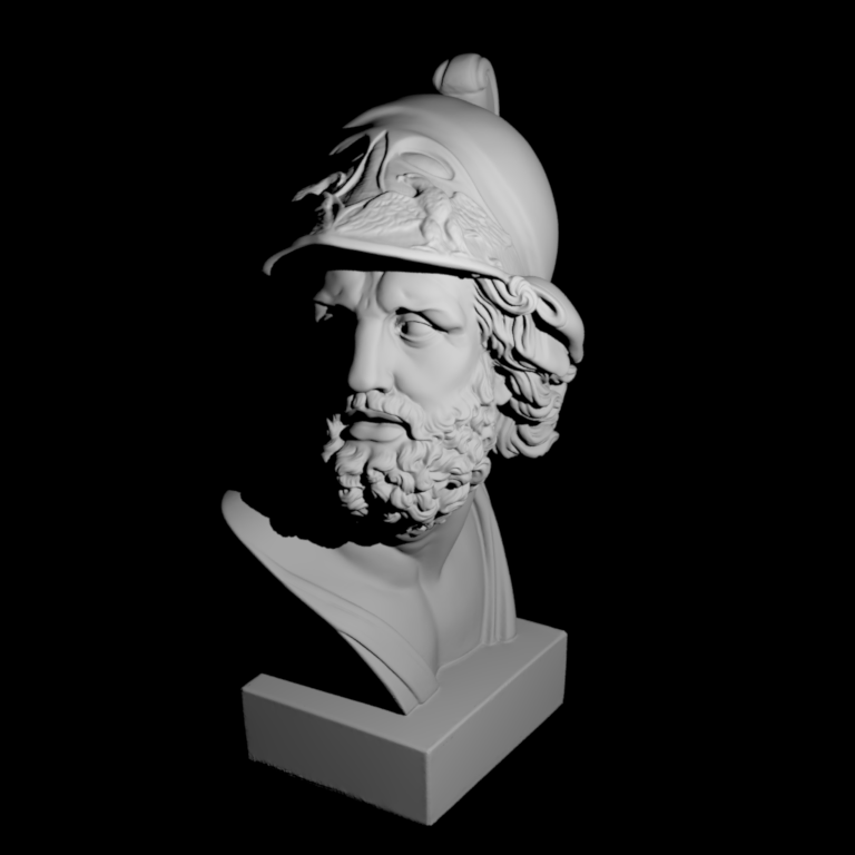
ajax-simple.xml 畫出來的圖,與題目提供的 reference image 看起來相同。實驗一下不同的 eps 值,會發現如果設定太小(例如 1e-5)的話,會有一些黑色斑點,推測是浮點數誤差造成 rayIntersect 誤判。可以用下圖來比較。
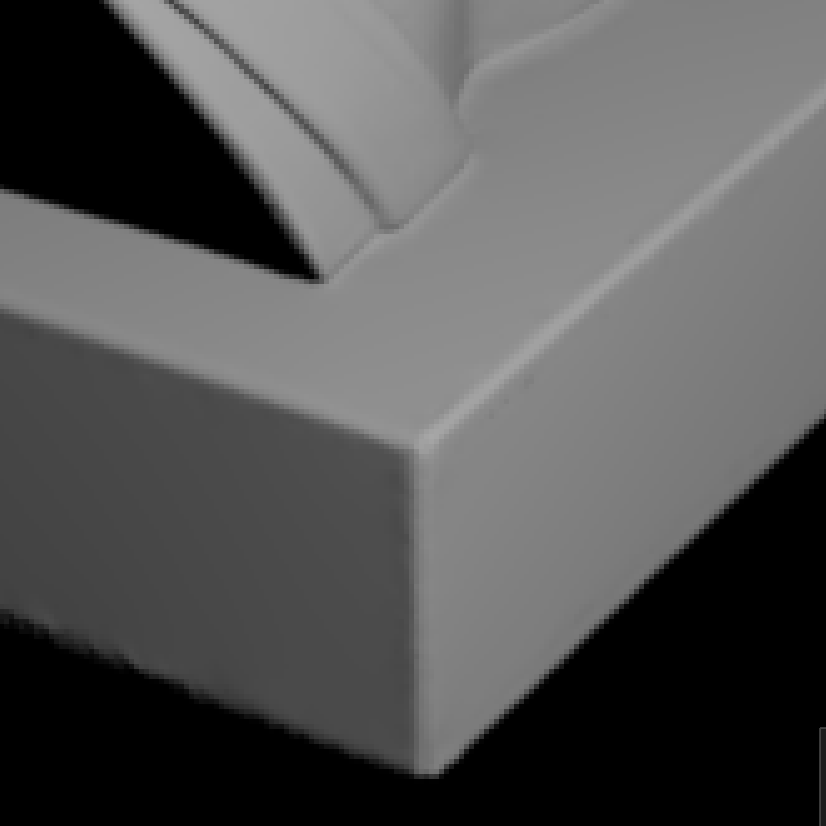
eps = 1e-3
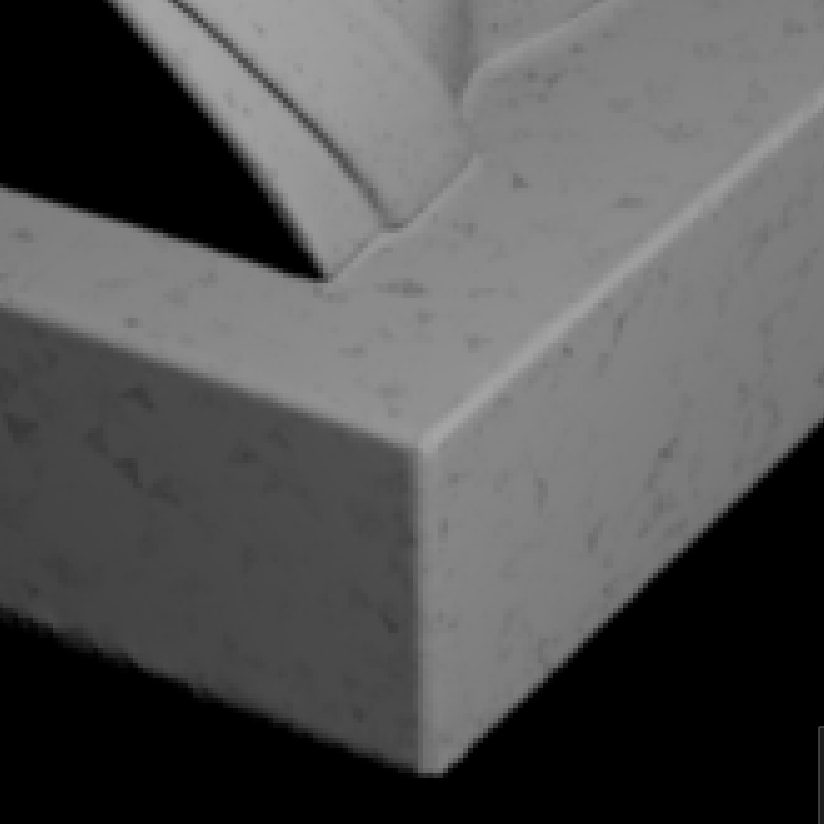
eps = 1e-5
ajax-simple.xml 的結果比較,不同 eps 值的影響。Part 2.2 Ambient Occlusion
一樣,把公式寫成 code 即可。
值得注意的是,Ray3f 如果不提供 mint 跟 maxt 的話,預設的值會是 epsilon 跟 infinity(見 include/nori/ray.h)。題目敘述中提到,我們可以把 $\alpha$ 設成 $\infty$,把 ambient occlusion 當成 global effect,因此使用 Ray3f constructor 預設的 mint 跟 maxt 即可。
    Color3f Li(const Scene *scene, Sampler *sampler, const Ray3f &ray) const {
        // find if the ray intersects with the scene
        Intersection its;
        if (!scene->rayIntersect(ray, its))
            return Color3f(0.0f);

        // use cosine weighted hemisphere sampling
        Vector3f direction = Warp::squareToCosineHemisphere(sampler->next2D());

        // use shadow ray query to obtain visibility
        Ray3f shadow_ray{its.p, its.shFrame.toWorld(direction)}; // (mint, maxt) = (eps, inf)
        return scene->rayIntersect(shadow_ray) ? 0.f : 1.f;
    }
在我的電腦上,./nori ajax-ao.xml 要跑 17 秒。
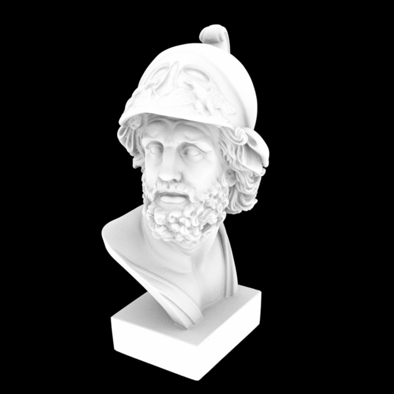
ajax-ao.xml 畫出來的圖,與題目提供的 reference image 看起來相同。錯誤嘗試(已折疊)
其實我原本寫的版本是自己在 Li() 裡面模擬積分,類似下方程式碼這樣,但這樣執行到天荒地老都跑不完。
    Color3f Li(const Scene *scene, Sampler *sampler, const Ray3f &ray) const {
        ...

        // simulate the integral
        Color3f ret{0.f};
        constexpr int num_sample = 1e3;
        for (int i = 0; i < num_sample; ++i) {
            // use cosine weighted hemisphere sampling
            Vector3f direction = Warp::squareToCosineHemisphere(Point2f{sampler->next2D()});

            // use shadow ray query to obtain visibility
            Ray3f shadow_ray{its.p, its.shFrame.toWorld(direction)}; // (mint, maxt) = (eps, inf)
            if (!scene->rayIntersect(shadow_ray)) {
                ret += 1.f;
            }
        }
        return ret / num_sample;
    }
後來發現,在 src/main.cpp 裡的 renderBlock() 中,可以看到對於每個 pixel,都會呼叫 sampler->getSampleCount() 次 integrator->Li()。也就是說,Monte Carlo averaging 已經發生在這邊了,我們不需要在 integrator 裡自己做積分的模擬。
    /* For each pixel and pixel sample sample */
    for (int y=0; y<size.y(); ++y) {
        for (int x=0; x<size.x(); ++x) {
            for (uint32_t i=0; i<sampler->getSampleCount(); ++i) {
                Point2f pixelSample = Point2f((float) (x + offset.x()), (float) (y + offset.y())) + sampler->next2D();
                Point2f apertureSample = sampler->next2D();

                /* Sample a ray from the camera */
                Ray3f ray;
                Color3f value = camera->sampleRay(ray, pixelSample, apertureSample);

                /* Compute the incident radiance */
                value *= integrator->Li(scene, sampler, ray);

                /* Store in the image block */
                block.put(pixelSample, value);
            }
        }
    }
後記
完成了 Assignment 2 了,很有趣。雖然機率跟微積分的數學有點令人力不從心,但還是感覺學到很多。電腦圖學最吸引我的地方,就是這樣把物理世界的公式,用非常漂亮的數學跟程式來表達和演算出來。看著自己的程式最終產生了想像中的圖,實在非常有成就感。
繼續往 Assignment 3 前進。